

Floyd-Warshall Takes the Wheel
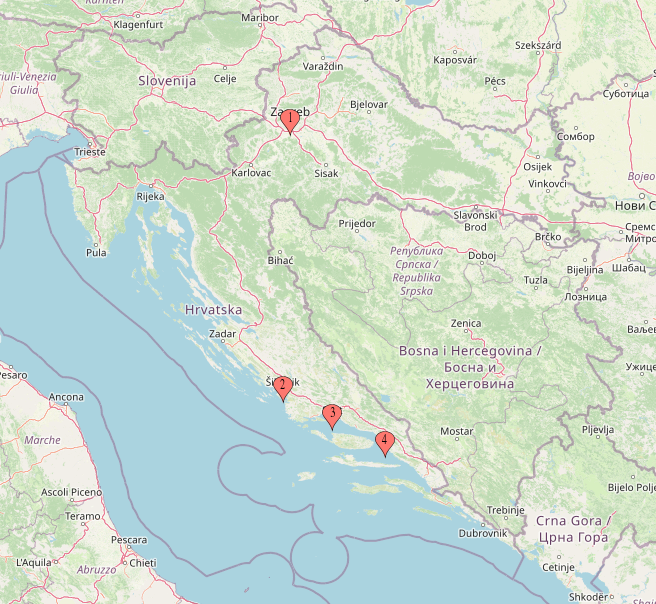
More than a month ago, I moved away from Zagreb. Summer had already started, it was getting hotter, so, naturally, my girlfriend and I wanted to go back to the coast where we could swim and enjoy overall more pleasant weather. We took a few trips:
- From Makarska, we went to Šibenik for a few days
- From Šibenik, we went to Makarska for a week, stopping at a shopping center in Split
- From Makarska, we went to Šibenik for about 10 days, driving a person from a ride-sharing app to a toll station near Split
- From Šibenik, we went to Makarska
Why are we talking about this?
Now you might be wondering why I’m telling you all of this? Who cares about my itinerary? Well, that’s what I would’ve thought as well, hadn’t I seen the image below. This is a screenshot of the ENC app. ENC stands for Elektronička naplata cestarine, or electronic toll collection in English. As you can see, I entered and exited a toll station 6 times.
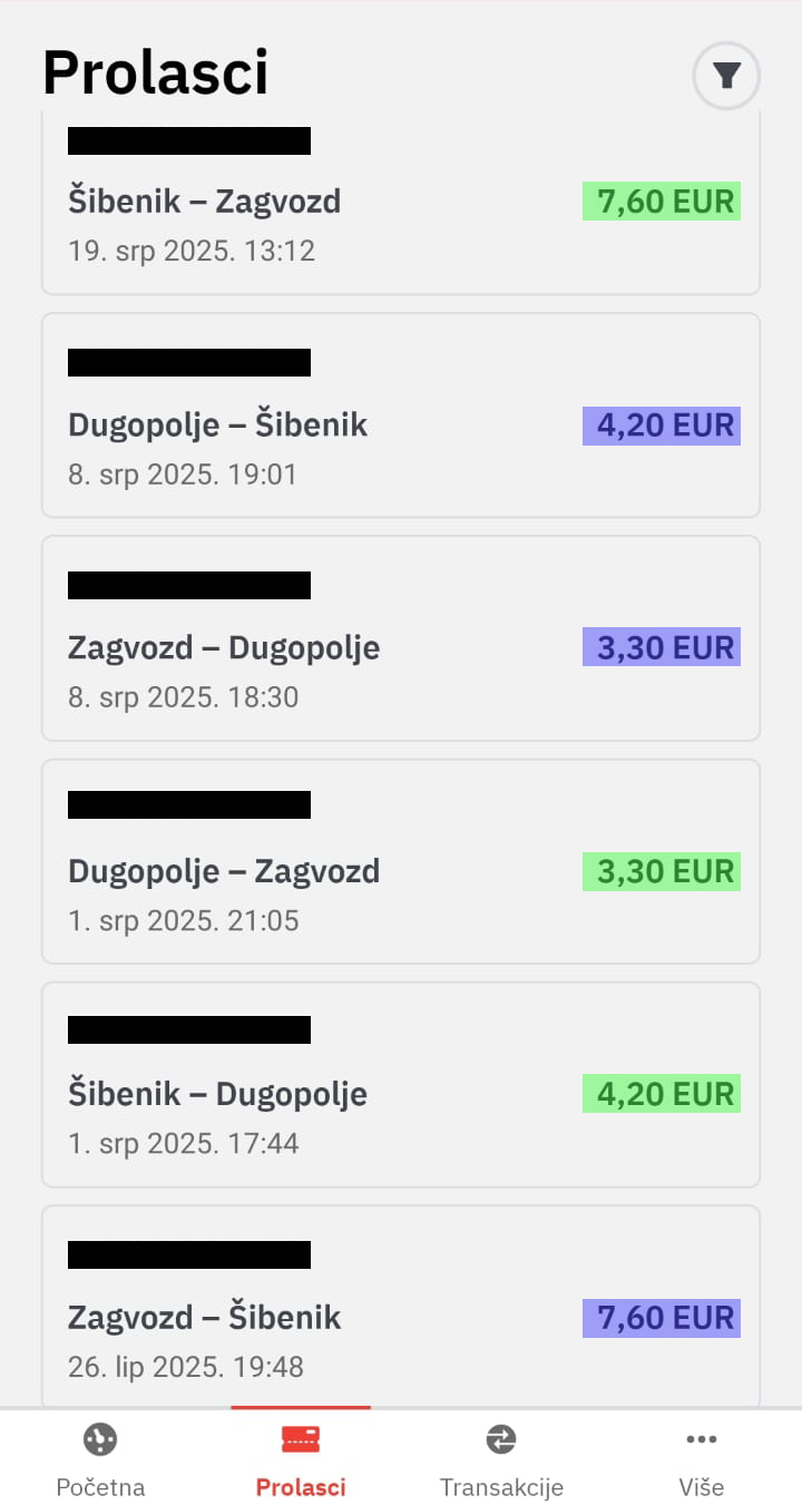
Do you notice anything weird in this image? From what it seems, when traveling from Šibenik to Zagvozd (a toll station near Makarska), it is ten cents cheaper to exit and re-enter at Dugopolje (a toll station near Split) than it is to drive directly. After seeing this, I was quite confused. Maybe this is a rounding error that happened when Croatia switched to the Euro? Surely that could explain a 10-cent difference? I had to investigate further.
Step 1: Gathering the Data
Of course, the first step was to get access to the prices between all pairs of toll stations. Luckily, Hrvatski autoklub (HAK, Croatian Automobile Club) got me covered. On their website, there is a price list, exactly what I needed.
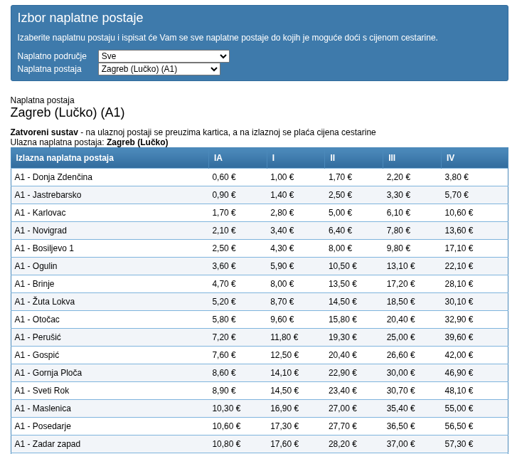
Hrvatske autoceste (HAC, Croatian Motorways) recognizes five vehicle categories, with each category having different toll charges:
- IA - Motorcycles
- I - Cars up to 1.90 meters in height
- II - Larger cars or cars with trailers
- III - Small trucks
- IV - Large trucks
After some simple network tab examination, I found the URL I needed to get access to all of the data programatically, so I set up a simple Python script that created an adjacency list between all pairs of connected toll stations for each vehicle category.
{
  "IA": {
    "A1_ZAGREB": {
      "name": "Zagreb (Lučko) (A1)",
      "connections": {
        "A1_DONJAZDENCINA": {
          "name": "Donja Zdenčina (A1)",
          "price": 0.6
        },
        "A1_JASTREBARSKO": {
          "name": "Jastrebarsko (A1)",
          "price": 0.9
        }
      }
    }
  }
}
Step 2: The Algorithm
Now, having all of the necessary data, I could use a modified version of the Floyd-Warshall algorithm to find and reconstruct the cheapest paths between all pairs of toll stations.
This algorithm is a good choice because it is easy to implement, and, even though it is slow ( where is the number of toll stations), the number of toll stations is small, and we’ll get the true cheapest paths, not approximations.
def floyd_warshall(
    self,
    dist: List[List[float]],
    next_station: List[List[Optional[str]]],
) -> Tuple[List[List[float]], List[List[Optional[str]]]]:
    """Apply Floyd-Warshall algorithm to find shortest paths"""
    n = len(dist)

    # Floyd-Warshall algorithm
    for k in range(n):
        for i in range(n):
            for j in range(n):
                if dist[i][k] + dist[k][j] < dist[i][j]:
                  dist[i][j] = dist[i][k] + dist[k][j]
                  next_station[i][j] = next_station[i][k]

    return dist, next_station
In simple terms, for each toll station , the algorithm updates the cheapest path between all pairs of toll stations on which a driver can use to exit and re-enter, and make the trip between and cheaper. It also stores the next station to exit on after , when driving from to . After running the algorithm, we get the cheapest paths between all connected pairs of toll stations, in a data structure like this:
{
  "A1_ZAGREB": {
    "name": "Zagreb (Lučko) (A1)",
    "destinations": {
      "A1_DONJAZDENCINA": {
        "name": "Donja Zdenčina (A1)",
        "shortest_price": 1.0,
        "path_stations": ["A1_ZAGREB", "A1_DONJAZDENCINA"],
        "path_names": ["Zagreb (Lučko) (A1)", "Donja Zdenčina (A1)"],
        "hops": 1,
        "original_direct_price": 1.0,
        "absolute_price_change": 0.0,
        "percentage_price_change": 0.0,
        "is_cheaper": false,
        "savings": 0
      },
      "A1_JASTREBARSKO": {
        "name": "Jastrebarsko (A1)",
        "shortest_price": 1.4,
        "path_stations": ["A1_ZAGREB", "A1_JASTREBARSKO"],
        "path_names": ["Zagreb (Lučko) (A1)", "Jastrebarsko (A1)"],
        "hops": 1,
        "original_direct_price": 1.4,
        "absolute_price_change": 0.0,
        "percentage_price_change": 0.0,
        "is_cheaper": false,
        "savings": 0
      }
    }
  }
}
Step 3: Data Analysis & Visualization
Now that we’ve calculated the cheapest paths, it’s time to compare them with the prices for direct trips and see if we’ve found anything interesting. Let’s start with some statistics:
| Category | Max Savings (€) | Max % Savings |
|---|---|---|
| IA | 1.8 | 37.50% |
| I | 2.4 | 37.04% |
| II | 3.6 | 39.02% |
| III | 5.4 | 36.51% |
| IV | 10.7 | 36.59% |
As you can see, since the large truck category (IV) has the largest prices, it also has the largest savings opportunities (in absolute terms). Let’s explore this category in more detail:
| Origin | Destination | Stops Between | Original Price (€) | New Price (€) | Price Change (€) |
|---|---|---|---|---|---|
| Zaprešić (A2) | Trakošćan (A2) | 2 | 30.1 | 19.4 | -10.7 |
| Lipovac (A3) | Bregana (A3) | 11 | 65.4 | 59.0 | -6.4 |
| Spačva (A3) | Bregana (A3) | 10 | 61.9 | 55.9 | -6.0 |
| Županja (A3) | Bregana (A3) | 9 | 58.1 | 52.4 | -5.7 |
| Babina Greda (A3) | Bregana (A3) | 8 | 55.1 | 49.8 | -5.3 |
Very nice! Although it’s possible to save more than 10 euros, it’s quite hard to do so because most of these require too many stops. Let’s find the largest price changes when only one exit and re-enter is needed between start and stop stations:
| Origin | Destination | Stop in Between | Original Price (€) | New Price (€) | Price Change (€) |
|---|---|---|---|---|---|
| Zaprešić (A2) | Krapina (A2) | Mokrice (A2) | 15.8 | 11.2 | -4.6 |
| Mokrice (A2) | Đurmanec (A2) | Krapina (A2) | 12.3 | 7.8 | -4.5 |
| Mokrice (A2) | Trakošćan (A2) | Krapina (A2) | 16.2 | 11.7 | -4.5 |
| Zaprešić (A2) | Začretje (A2) | Mokrice (A2) | 13.5 | 10.3 | -3.2 |
| Začretje (A2) | Đurmanec (A2) | Krapina (A2) | 6.5 | 5.3 | -1.2 |
Even better! As we can see, the A2 highway offers some significant savings with just one stop! Let’s see the one-stop data for IA and I categories, as they are the most relevant categories for the most people:
IA Category
| Origin | Destination | Stop in Between | Original Price (€) | New Price (€) | Price Change (€) |
|---|---|---|---|---|---|
| Zaprešić (A2) | Krapina (A2) | Mokrice (A2) | 2.1 | 1.5 | -0.6 |
| Mokrice (A2) | Đurmanec (A2) | Krapina (A2) | 1.6 | 1.0 | -0.6 |
| Zaprešić (A2) | Začretje (A2) | Mokrice (A2) | 1.8 | 1.4 | -0.4 |
| Tunel Učka/Matulji (A8) | Žminj (A8) | Vranja (A8) | 5.3 | 5.0 | -0.3 |
| Donja Zdenčina (A1) | Bosiljevo 1 (A1) | Novigrad (A1) | 2.0 | 1.8 | -0.2 |
I Category
| Origin | Destination | Stop in Between | Original Price (€) | New Price (€) | Price Change (€) |
|---|---|---|---|---|---|
| Zaprešić (A2) | Krapina (A2) | Mokrice (A2) | 3.5 | 2.5 | -1.0 |
| Mokrice (A2) | Đurmanec (A2) | Krapina (A2) | 2.7 | 1.7 | -1.0 |
| Mokrice (A2) | Trakošćan (A2) | Krapina (A2) | 3.6 | 2.6 | -1.0 |
| Zaprešić (A2) | Začretje (A2) | Mokrice (A2) | 3.0 | 2.3 | -0.7 |
| Tunel Učka/Matulji (A8) | Žminj (A8) | Vranja (A8) | 8.8 | 8.4 | -0.4 |
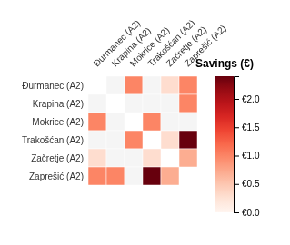
To end this blog post, I made interactive heatmaps showing price changes both in euro amounts and percentages for each of the vehicle categories and highways. Below are the screenshots for the I vehicle category on the A1-A6 connection and the A2 highway.
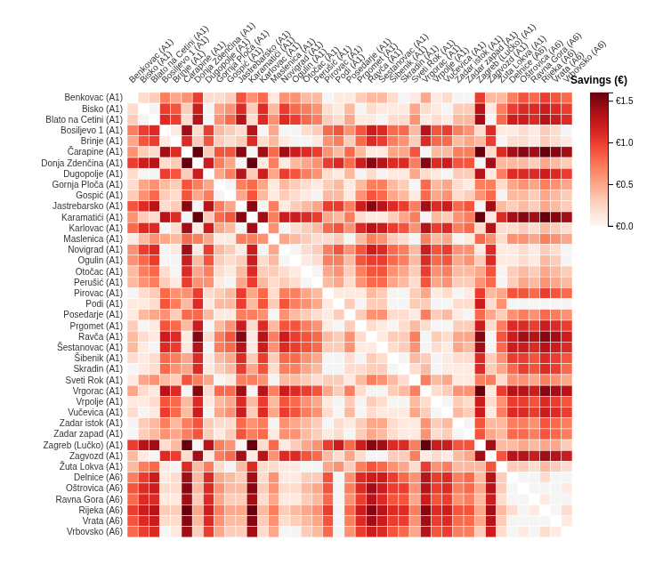
All of the code, data, and many more visualizations are available in this repository, although I must say that the code is messy because it was mostly vibe-coded. The JSON files are quite nice, though, and I would love to see if you can extract any cool insights from them!